Bài viết này sẽ trình bày việc tính toán động lực học tay máy phẳng 2 bậc tự do. Quá trình tính toán phương trình động lực học sử dụng bằng Matlab symbolics để tính toán với các biến số. Sau khi tìm được phương trình động lực học thì bài viết sẽ hướng dẫn sử dụng bộ điều khiển PID để điều khiển tay máy di chuyển từ vị trí ban đầu đến vị trí mong muốn. Kết quả mô phỏng cho thấy sai số hội tụ về 0 và cho thấy giá trị torque mà động cơ tại mỗi khớp cần cung cấp. Cuối cùng bài viết sẽ cung cấp toàn bộ code Matlab dùng để mô phỏng.
Phương trình động lực học
Giả sử tay máy có thông số như hình vẽ
Vị trí của khối lượng m1 và m2 lần lượt là (x1,y1) và (x2,y2). Chúng ta dễ dàng tính được:
function xdot=r2dof(t,x,ths,spec,Kpid)xdot=zeros(8,1);%% set-pointsth1s=ths(1);th2s=ths(2);%% Robot SpecificationsM1=spec(3);M2=spec(4);L1=spec(1);L2=spec(2);g=9.8;%% Inertia Matrixb11=(M1+M2)*L1^2+M2*L2^2+2*M2*L1*L2*cos(x(4));b12=M2*L2^2+M2*L1*L2*cos(x(4));b21=M2*L2^2+M2*L1*L2*cos(x(4));b22=M2*L2^2;Bq=[b11 b12;b21 b22];%% C Matrixc1=-M2*L1*L2*sin(x(4))*(2*x(5)*x(6)+x(6)^2);c2=-M2*L1*L2*sin(x(4))*x(5)*x(6);Cq=[c1;c2];%% Gravity Matrixg1=-(M1+M2)*g*L1*sin(x(3))-M2*g*L2*sin(x(3)+x(4));g2=-M2*g*L2*sin(x(3)+x(4));Gq=[g1;g2];%% PID Control% PID parameters for theta 1Kp1=Kpid(1);Kd1=Kpid(2);Ki1=Kpid(3);% PID parameters for theta 2Kp2=Kpid(4);Kd2=Kpid(5);Ki2=Kpid(6);%decoupled control inputf1=Kp1*(th1s-x(3))-Kd1*x(5)+Ki1*(x(1));f2=Kp2*(th2s-x(4))-Kd2*x(6)+Ki2*(x(2));Fhat=[f1;f2];F=Bq*Fhat;% actual input to the system%% System statesxdot(1)=(th1s-x(3));%dummy state of theta1 integrationxdot(2)=(th2s-x(4));%dummy state of theta2 integrationxdot(3)=x(5);%theta1-dotxdot(4)=x(6);%theta2-dotq2dot=Bq\(-Cq-Gq+F);xdot(5)=q2dot(1);%theta1-2dotxdot(6)=q2dot(2);%theta1-2dot%control input function output to outside computer programxdot(7)=F(1);xdot(8)=F(2);
Code main
close all
clear all
clc
%% Initilizationth_int=[-pi/2pi/2];%initial positionsths=[pi/2-pi/2];%set-pointsx0=[00 th_int 0000];%states initial valuesTs=[020];%time span%% Robot SpecificationsL1=1;%link 1L2=1;%link 2M1=1;%mass 1M2=1;%mass 2spec=[L1 L2 M1 M2];%% PID Parameters% PID parameters for theta 1Kp1=15;Kd1=7;Ki1=10;% PID parameters for theta 2Kp2=15;Kd2=10;Ki2=10;Kpid=[Kp1 Kd1 Ki1 Kp2 Kd2 Ki2];%% ODE solving% opt1=odeset('RelTol',1e-10,'AbsTol',1e-20,'NormControl','off');[T,X]=ode45(@(t,x)r2dof(t,x,ths,spec,Kpid),Ts,x0);%% Outputth1=X(:,3);%theta1 wavwformth2=X(:,4);%theta2 wavwform%torque inputs computation from the 7th,8th states inside ODEF1=diff(X(:,7))./diff(T);F2=diff(X(:,8))./diff(T);tt=0:(T(end)/(length(F1)-1)):T(end);%xyx1=L1.*sin(th1);% X1y1=L1.*cos(th1);% Y1x2=L1.*sin(th1)+L2.*sin(th1+th2);% X2y2=L1.*cos(th1)+L2.*cos(th1+th2);% Y2%theta1 error plotplot(T,ths(1)-th1)grid
title('Theta-1 error')ylabel('theta1 error (rad)')xlabel('time (sec)')%theta2 error plotfigure
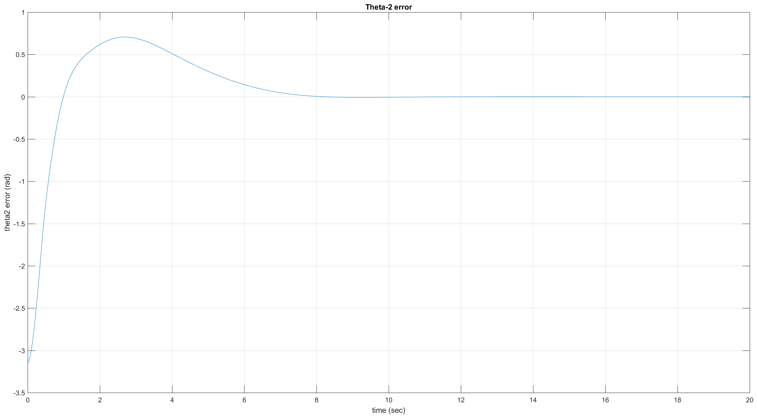
plot(T,ths(2)-th2)grid
title('Theta-2 error')ylabel('theta2 error (rad)')xlabel('time (sec)')%torque1 plotfigure
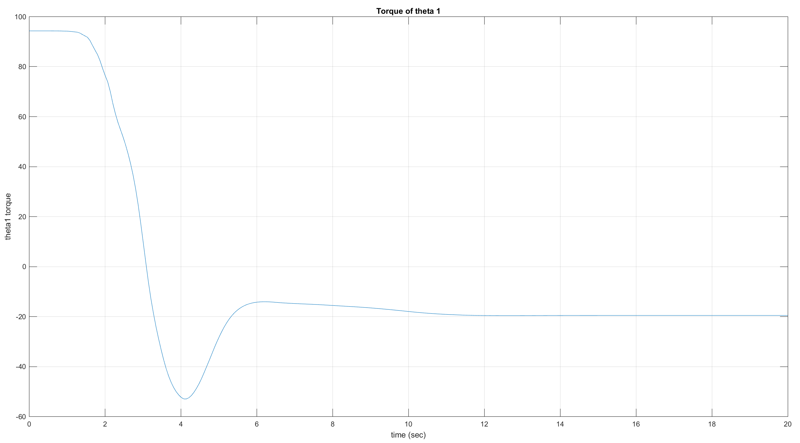
plot(tt,F1)grid
title('Torque of theta 1')ylabel('theta1 torque')xlabel('time (sec)')%torque2 plotfigure
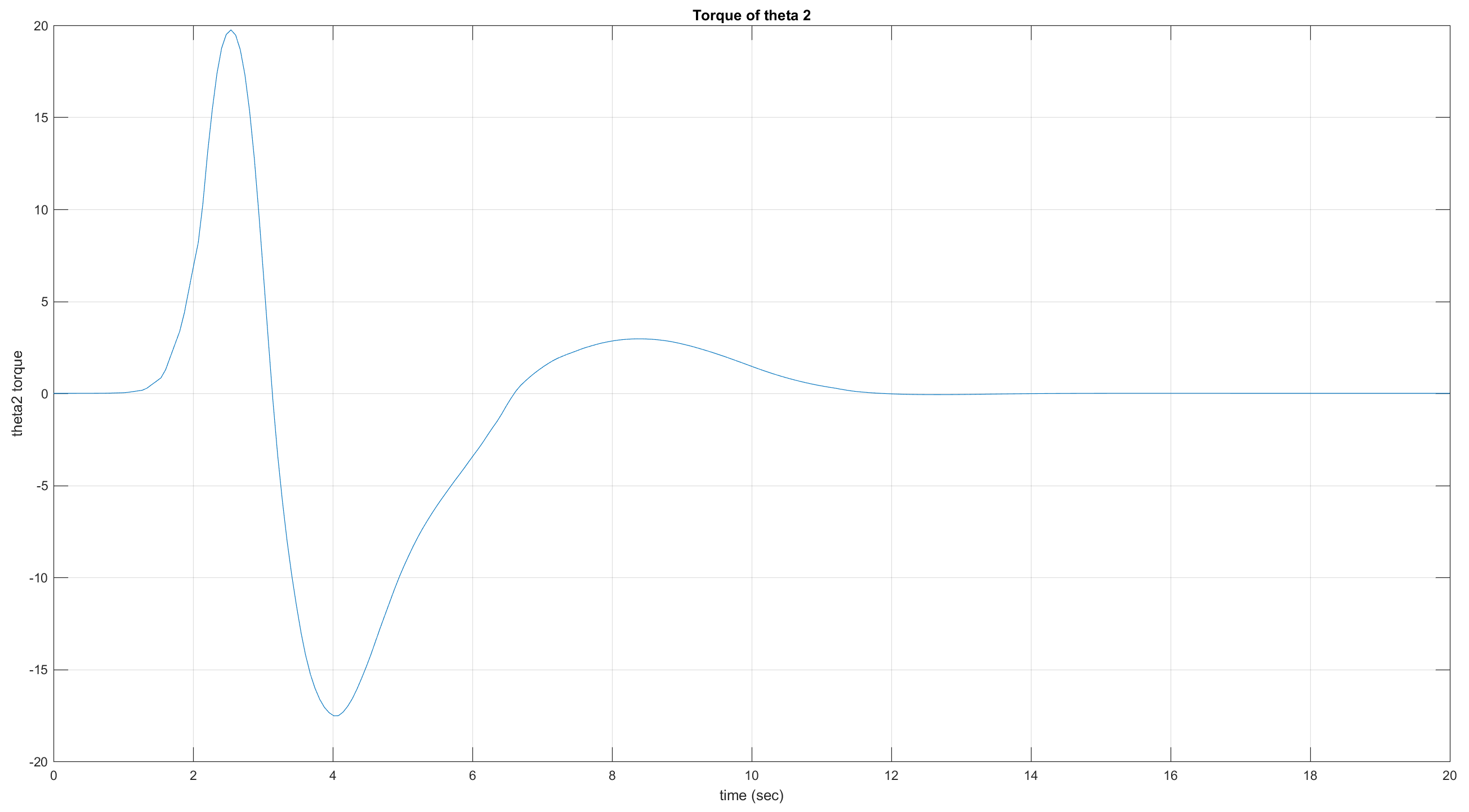
plot(tt,F2)grid
title('Torque of theta 2')ylabel('theta2 torque')xlabel('time (sec)')
Code animation
%% setting frames speedd=2;j=1:d:length(T);%% generating images in 2Dfigure
vd =VideoWriter('2DOF_rob.avi');open(vd);fori=1:length(j)-1hold off
plot([x1(j(i))x2(j(i))],[y1(j(i))y2(j(i))],'o',[0x1(j(i))],[0y1(j(i))],'k',[x1(j(i))x2(j(i))],[y1(j(i))y2(j(i))],'k')title('Motion of 2DOF Robotic Arm')xlabel('x')ylabel('y')axis([-33-33]);grid
hold on
drawnow;frame = getframe;writeVideo(vd,frame);endclose(vd);